Behind the Model
The purpose of this page is to provide a detailed explanation of how the backend model works and develop an understanding of where the model may fail. An understanding of linear algebra and calculus will be helpful.
Overview
The core thesis of this project is that public equity performance is influenced by a complex array of market conditions and financial composition. By training a neural network to model one-year equity yield using extensive historical data, we gain a method to decode these underlying complexities. Although it is impossible to predict the future, the benefit of this approach is that it is not dependent on predicting portfolio yield with 100% accuracy - but is successful if it is able quantify uncertainty and provide guidance on how to manage and limit risk exposure. This is achieved by training the neural network to estimate a confidence interval rather than a point estimate, allowing for a more robust interpretation of potential outcomes. Additionally, training at portfolio level (rather than individual securities) enables more effective risk mitigation through diversification and allows the model to capture cointegrated relationships between assets, which can further stabilize returns.
Limitations
When reviewing the results, it is important to consider the limitations of the prediction model. Understanding these constraints provides better context for where
predictions may fall short and how additional research can complement the statistical outputs.
Company Financials:
The model is not directly trained on underlying financial reporting metrics such as balance sheet, income statement, or cash flow data. As a result, it may not fully
capture company-specific structural risks that are not reflected in equity pricing. Users are encouraged to review financial statements and conduct independent analysis
of key financial indicators.
Social Perception & Media Influence:
While the model incorporates proxy variables such as trading volume trends, it does not capture shifts in public perception driven by news or media. These factors are
inherently difficult to quantify but can materially impact investment performance. Users should incorporate qualitative judgment regarding market sentiment and media
narratives.
Data Quality:
The model relies on publicly available APIs for both training and prediction data, including sources such as Yahoo Finance, the Bank of Canada, Statistics Canada, and
the Federal Reserve Economic Data (FRED). As with any live data feed, there is an inherent risk of inaccuracies or delays.
Sector Classification for ETFs:
Current data sources do not provide precise sector classifications for ETFs. Consequently, ETFs are treated as a generalized sector category rather than being mapped
to specific industries (e.g., energy, financials, technology). This limitation arises because many ETFs span multiple sectors, making dynamic classification unreliable.
While this reduces granularity, other controls—such as product type, dividend characteristics, and risk profile—help maintain the robustness of the analysis.
Building the prediction model
The first 'learning' stage of this model is based on a regression trained neural net aiming to predict portfolio yield.
The purpose of this step is to generate a function N() which can predict how a portfolio will perform given
a set of conditions (composition, market features, economic data etc.). Instead of building a predetermined function which
may theoretically represent portfolio perfomance, this approach allows the neural net to act as a functional representation of the market
and dynamically adjust to real performance from over 500k random portfolios from different industries, time periods & compositional characteristics. Additionally,
when programming the neural net pipeline ensuring differentiability, it allows for the calculation of gradients which is the primary means
of optimizing the allocation within a specific portfolio.
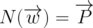
where:
- N = Neural network
- w = Security distribution vector
- P = Performance vector
* Side note: In actual implementation, the weight vector is not passed directly into the network but is passed
through a series of preprocessing functions. For simplicity I will just show the w vector as a direct input. In reality
it would look something like the following:

Portfolio optimization
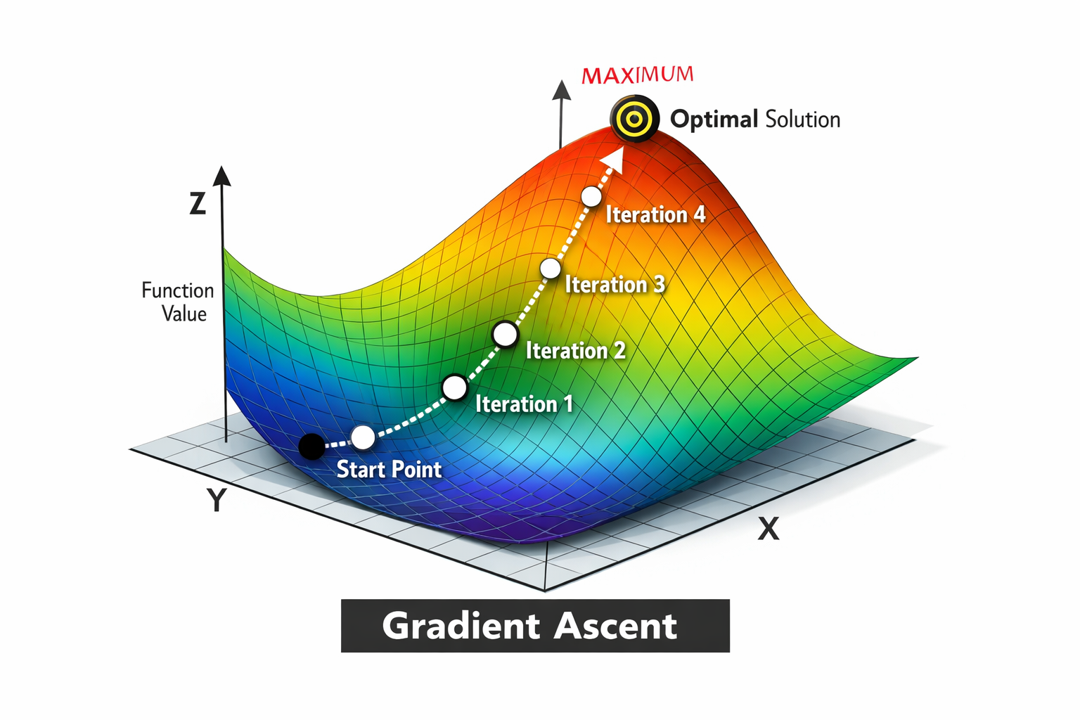
Once the neural net is trained, functional representation is used so that the model can 'learn' how to optimize performance by changing the input allocation vector (w). This process is done through gradient ascent:
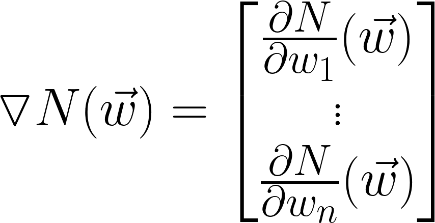
Gradient Vector Calculation
1 step in learning
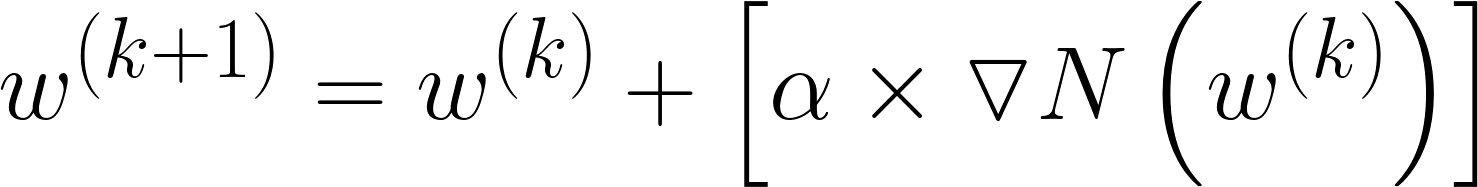
- N = Neural network
- w = Security distribution vector
- a = alpha (learning rate) - scaling for gradient vector
- k = iteration
Example visual:
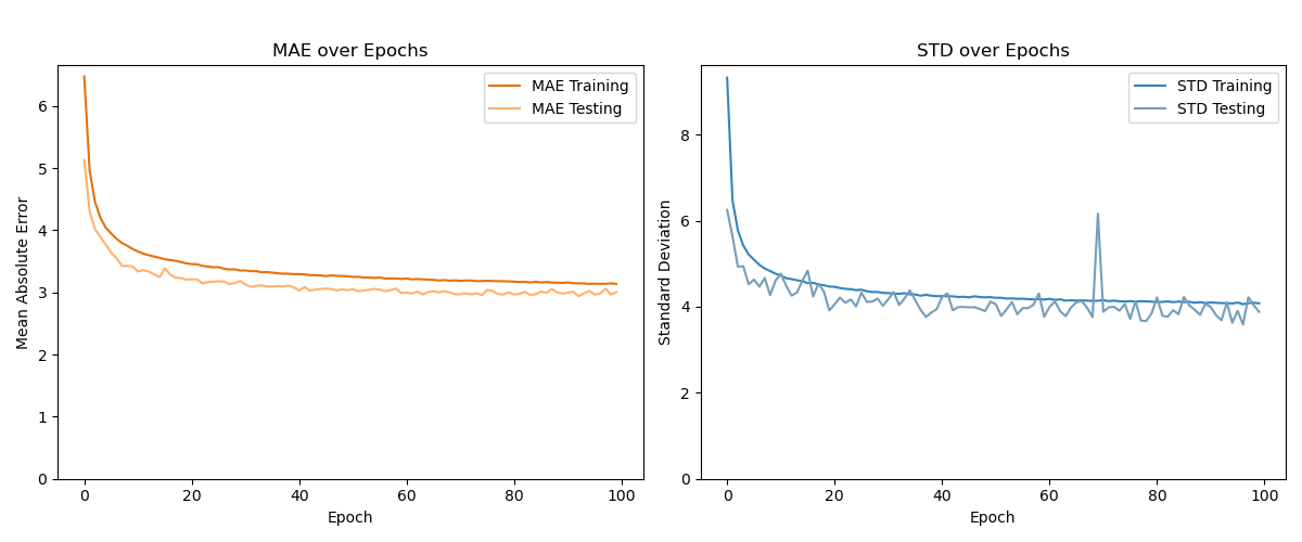
Network Training Results
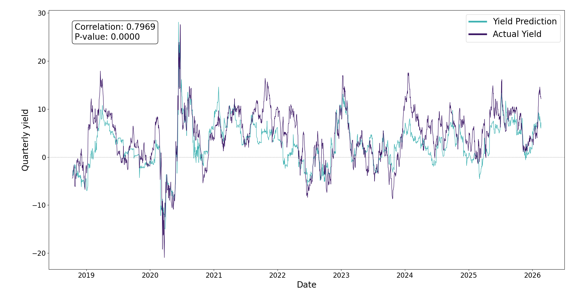
Network Yield Predictions vs Real Performance
The following graph shows the annual yield prediction from the network compared to the actual portfolio yield. Predictions are made on data prior to the performance window - mimicking current day application.
- Royal Bank of Canada (20%)
- Canadian National Railway (20%)
- Enbridge Inc. (20%)
- Loblaw Co. (20%)
- Maple Leaf Foods (20%)
Neural Net - Additional info
Structure
Hidden Nodes: Each hidden node in the network is 'connected' to each node in the adjacent layers. The term connected means the following:
- The node recieves the outputs from all nodes in the previous layer (as a vector) and applies some transformation to it. Ex:
f(V) = transformed scalar - The output of the node is used as an element in a vector passed along to the nodes in the next layer. Ex:
V = [f(V1),f(V2),f(V3),...,f(Vn)]f(V) = another transformed scalar
Note: Each node in the hidden layers acts as a feature identifier, which is what allows the network to 'learn' highly complex patterns. For example, if the first node in the first hidden layer has assigned weights which focus on identifying when a portfolio has high inflation, high price volatility and high beta, it will then return a stronger signal output >> f(V) << when that case presents itself. This signal output is then passed along to the next layer. In the second layer the signal recieved from node 1 along with the signals recieved from all other nodes (each trained to identify distinct features) will be used to analyze relationships between various signal outputs and assign weights to identify 'deeper' patterns - hense the term deep learning.
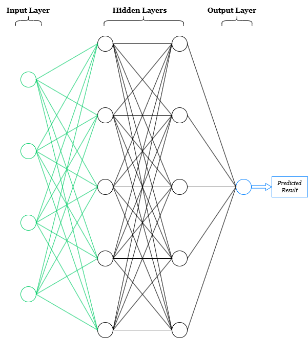
Input Nodes: The input layer gets scaled first (keras normalization) then each column/feature in the dataset is passed on as a distinct node.
Output Node: The output layer applies a final transformation from the nodes in the final hidden layer to return 1 predicted result.
Individual Node - transformation & activation
There are two main operations which happen within each node:
- Transformation
- Activation
- Transformation -
So far, the transformation function has been written in a generic format: f(V). The actual function used on each node is the following:
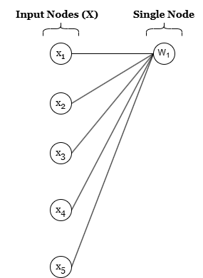
f(V) = W * X + b
where W * X is the dot product of two vectors and b is a bias scalar to
introduce unbounded mapping (will not need to pass through origin [0,0,...0]). W and b are
gradually 'learned' through network passes and X is the vector of signals recieved from the
previous layer as described above.
W = [w1, w2, w3, ..., wn]
X = [x1, x2, x3, ..., xn]
- Activation -
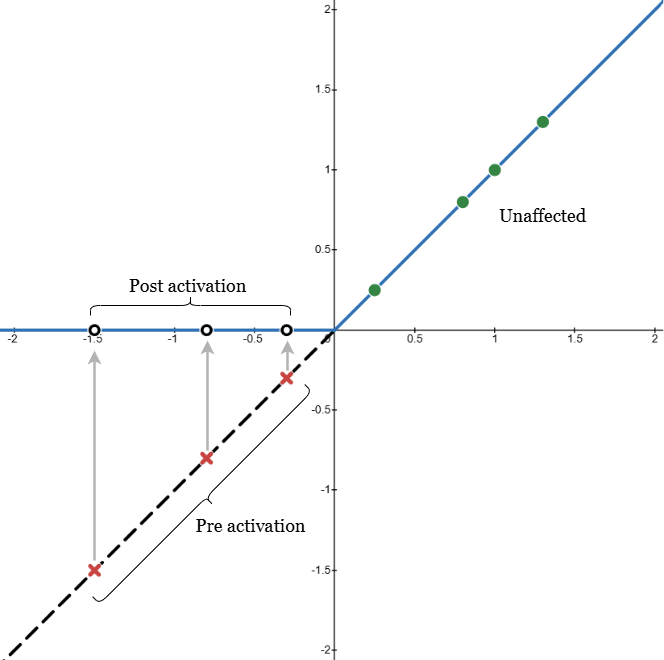
Activation is required to introduce non-linarity into the network. Without an activation function the network could be reduced down to a series of linear transformations - which is limited. Conceptually, activation is designed as a 'switch' so that a signal will only be returned from a node if the distinct feature is identified (see note section above describing node features). The activation function used in this project is ReLU (Rectified Linear Unit):
ReLU = max(0, f(V))
The benefit with ReLU activiation is that aside from begin a switch (binary indicator of feature presence) it indicates signal strength when the features are present - allowing for more rigorous analysis. The graph to the right shows examples of how transformation results would be treated before & after activation. The points with a red X show the 'pre activation' result which after activation return a muted signal (0) for that node (empty black circles). Only the green circles are passed on to the network. The signal strength of the node (if not muted) is dependent on the magnitude of the transformed output. This function is what allows nodes to be feature specific and map characteristics of complex inputs.