Quantitative Portfolio Analysis

# Portfolio Optimization
import os
os.environ['TF_CPP_MIN_LOG_LEVEL'] = '1'  # or '3' to suppress even more

import matplotlib.pyplot as plt
import pandas as pd
import yfinance as yf
from dateutil.relativedelta import relativedelta
from tqdm import tqdm

from SpecificPortfolio.Training import Model
from TrainingSet import Data as Source


# See README file for project description

# _____________________MODEL INPUTS________________________
# >List of Securities
Securities1 = ['RY.TO', 'CNQ.TO', 'TD.TO', 'CM.TO', 'ENB.TO', 'SU.TO', 'BNS.TO', 'TRP.TO', 'AEM.TO', 'NTR.TO']
ETF1 = 'ZWC.TO'

Securities2 = ['SU.TO', 'ENB.TO', 'NA.TO', 'FTS.TO', 'TD.TO', 'CM.TO', 'GWO.TO', 'RY.TO', 'BMO.TO', 'CNR.TO']
ETF2 = 'XMV.TO'

Securities3 = ['RY.TO', 'TD.TO', 'SHOP.TO', 'AEM.TO', 'ENB.TO', 'BMO.TO', 'BN.TO', 'CM.TO', 'BNS.TO', 'CNQ.TO']
ETF3 = 'VCN.TO'

Securities4 = ['CLS.TO', 'SHOP.TO', 'CSU.TO', 'GIB-A.TO', 'DSG.TO', 'OTEX.TO', 'KXS.TO', 'BB.TO', 'LSPD.TO', 'BITF.TO']
ETF4 = 'XIT.TO'

Quarters = 10
InitialBudget = 1000
MaxSteps = 100  # <- Number of vector steps the model will go through until end of optimization

GROUPS = [
    {"name": "Group 1", "securities": Securities1, "etf": ETF1},
    {"name": "Group 2", "securities": Securities2, "etf": ETF2},
    {"name": "Group 3", "securities": Securities3, "etf": ETF3},
    {"name": "Group 4", "securities": Securities4, "etf": ETF4},
]


def build_etf_value(etf_ticker, quarters, budget):
    data = yf.Ticker(etf_ticker).history(period="max")[['Close', 'Dividends']]
    data.index = pd.to_datetime(data.index)
    data = data.sort_index()

    end_filter = data.index[-1] - pd.DateOffset(months=3 * quarters)
    df_filtered = data[data.index > end_filter].copy()
    quarterly_dates = df_filtered.index[::63]

    dividend_payouts = df_filtered[df_filtered["Dividends"] > 0].copy()

    initial_shares = budget / df_filtered['Close'].iloc[0]
    current_shares = initial_shares
    running_shares = []

    # Accounts for compounding dividends through additional share purchases.
    for _, row in dividend_payouts.iterrows():
        div_shares = current_shares * row['Dividends'] / row['Close']
        running_shares.append(div_shares)
        current_shares += div_shares

    dividend_payouts["DivPayouts"] = running_shares

    df = df_filtered.copy()
    df["DivPayouts"] = dividend_payouts["DivPayouts"].reindex(df.index, fill_value=0)
    df.iloc[0, df.columns.get_loc("DivPayouts")] += initial_shares
    df['cum_Shares'] = df['DivPayouts'].cumsum()
    etf_value = df['Close'] * df['cum_Shares']

    return etf_value, quarterly_dates


def run_group(group, quarters, initial_budget, max_steps):
    securities = group["securities"]
    etf = group["etf"]

    etf_value, quarterly_dates = build_etf_value(etf, quarters, initial_budget)

    model = Model(securities, max_steps)
    calc_obj = model.CalcObj

    optimized_value = []
    budget = initial_budget
    dataset, _, dividends, _ = Source.yf_Data(securities)

    # Quarterly adjustments.
    for quarter_date in tqdm(quarterly_dates.tz_localize(None), desc=group["name"]):
        date_input = quarter_date + relativedelta(months=3)  # aligns with calc obj processing
        calc_obj.Specify(date_input, securities)
        model.Features = calc_obj

        weights = model.Train()  # <= optimal weight for next quarter

        dataset_filtered = dataset[(dataset.index > quarter_date) & (dataset.index < date_input)]
        dividends_filtered = dividends[(dividends.index > quarter_date) & (dividends.index < date_input)]

        indv_alloc = weights * budget
        shares = indv_alloc / dataset_filtered.iloc[0]
        portfolio = (dataset_filtered * shares).sum(axis=1)
        divs = (dividends_filtered * shares).sum().sum()  # total dividends over the quarter

        # Budget at end of quarter will be ending capital plus accumulated dividends.
        budget = portfolio.iloc[-1] + divs

        # Add dividends accumulated to end-of-quarter portfolio value.
        portfolio.loc[portfolio.index[-1]] += divs
        optimized_value.append(portfolio)

    total_value = pd.concat(optimized_value)

    optimized_return = (total_value.iloc[-1] - total_value.iloc[0]) / total_value.iloc[0]
    optimized_quarterly = ((1 + optimized_return) ** (1 / quarters) - 1) * 100

    etf_return = (etf_value.iloc[-1] - etf_value.iloc[0]) / etf_value.iloc[0]
    etf_quarterly = ((1 + etf_return) ** (1 / quarters) - 1) * 100

    total_value.index = total_value.index.tz_localize(None) if total_value.index.tz else total_value.index
    etf_value.index = etf_value.index.tz_localize(None) if etf_value.index.tz else etf_value.index

    return {
        "name": group["name"],
        "etf": etf,
        "securities": securities,
        "total_value": total_value,
        "etf_value": etf_value,
        "optimized_quarterly": optimized_quarterly,
        "etf_quarterly": etf_quarterly,
    }


def plot_group_comparison(results):
    fig, axes = plt.subplots(2, 2, figsize=(18, 12), sharex=False, sharey=False)
    axes = axes.flatten()

    for ax, result in zip(axes, results):
        total_value = result["total_value"]
        etf_value = result["etf_value"]

        ax.plot(total_value.index, total_value.values, label='True North Portfolio Research', color='blue')
        ax.plot(etf_value.index, etf_value.values, label=result["etf"], color='orange')

        ax.text(
            total_value.index[-1],
            total_value.values[-1],
            f"Avg Qrtly Return {result['optimized_quarterly']:.2f}%",
            color='blue',
            va='center',
            ha='left',
            fontsize=10,
            bbox=dict(facecolor='white', edgecolor='black', boxstyle='round,pad=0.3')
        )

        ax.text(
            etf_value.index[-1],
            etf_value.values[-1],
            f"Avg Qrtly Return {result['etf_quarterly']:.2f}%",
            color='orange',
            va='center',
            ha='left',
            fontsize=10,
            bbox=dict(facecolor='white', edgecolor='black', boxstyle='round,pad=0.3')
        )

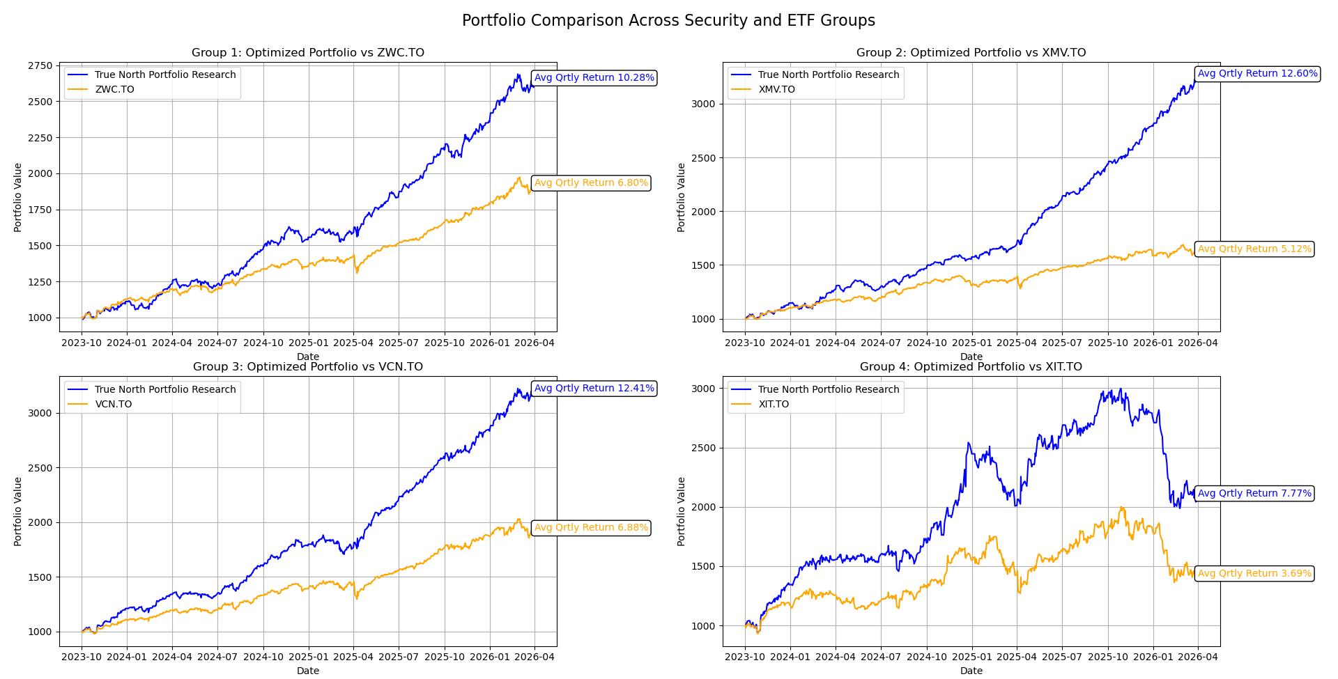
        ax.set_title(f"{result['name']}: Optimized Portfolio vs {result['etf']}")
        ax.set_xlabel('Date')
        ax.set_ylabel('Portfolio Value')
        ax.grid(True)
        ax.legend()

    for ax in axes[len(results):]:
        ax.remove()

    fig.suptitle('Portfolio Comparison Across Security and ETF Groups', fontsize=16)
    fig.tight_layout(rect=[0, 0, 1, 0.97])
    plt.show()


all_results = [run_group(group, Quarters, InitialBudget, MaxSteps) for group in GROUPS]
plot_group_comparison(all_results)